1 线性回归
重点概念:
线性回归(linear regression)、标签(label)或目标(target)、特征(feature)或协变量(covariate)、权重(weight)、偏置(bias)、偏移量(offset)或截距(intercept)、解析解(analytical solution)、调参(hyperparameter tuning)、泛化(generalization)、正态分布(normal distribution)或高斯分布(Gaussian distribution)、似然(likelihood)
线性模型可以看作是单层的神经网络
仿射变换(affine transformation):线性变换和平移变换的叠加
梯度下降(gradient descent):沿着反梯度方向更新参数寻找最优解
小批量随机梯度下降(minibatch stochastic gradient descent):在梯度下降的基础上的优化,寻求并行计算量和内存消耗的平衡
两个重要的超参数(hyperparameter):批量大小(batch size)、学习率(learning rate)
矢量化加速:并行计算的代码通常会带来数量级的加速
最小化目标函数和执行极大似然估计是等价的
2 线性回归实现(pytorch)
2.1 从零开始版本
%matplotlib inline
import random
import torch
from d2l import torch as d2l

def synthetic_data(w, b, num_examples):
    """生成 y = Xw + b + 噪声。"""
    X = torch.normal(0, 1, (num_examples, len(w)))
    y = torch.matmul(X, w) + b
    y += torch.normal(0, 0.01, y.shape)
    return X, y.reshape((-1, 1))

true_w = torch.tensor([2, -3.4])
true_b = 4.2
features, labels = synthetic_data(true_w, true_b, 1000)

print('features:', features[0], '\nlabel:', labels[0])
# features: tensor([-0.6612, -1.8215])
# label: tensor([9.0842])

def data_iter(batch_size, features, labels):
    """定义数据迭代器"""
    num_examples = len(features)
    indices = list(range(num_examples))
    random.shuffle(indices)
    for i in range(0, num_examples, batch_size):
        batch_indices = torch.tensor(indices[i:min(i +
                                                   batch_size, num_examples)])
        yield features[batch_indices], labels[batch_indices]

batch_size = 10

# 定义 初始化模型参数
w = torch.normal(0, 0.01, size=(2, 1), requires_grad=True)
b = torch.zeros(1, requires_grad=True

# 定义模型
def linreg(X, w, b):
    """线性回归模型。"""
    return torch.matmul(X, w) + b

# 定义损失函数
def squared_loss(y_hat, y):
    """均方损失。"""
    return (y_hat - y.reshape(y_hat.shape))**2 / 2

# 定义优化算法
def sgd(params, lr, batch_size):
    """小批量随机梯度下降。"""
    with torch.no_grad():
        for param in params:
            param -= lr * param.grad / batch_size
            param.grad.zero_()

# 训练过程
lr = 0.03
num_epochs = 3
net = linreg
loss = squared_loss

for epoch in range(num_epochs):
    for X, y in data_iter(batch_size, features, labels):
        l = loss(net(X, w, b), y)
        l.sum().backward()
        sgd([w, b], lr, batch_size)
    with torch.no_grad():
        train_l = loss(net(features, w, b), labels)
        print(f'epoch {epoch + 1}, loss {float(train_l.mean()):f}')
# epoch 1, loss 0.033103
# epoch 2, loss 0.000124
# epoch 3, loss 0.000054

# 比较真实参数和通过训练学到的参数来评估训练的效果
print(f'w的估计误差: {true_w - w.reshape(true_w.shape)}')
print(f'b的估计误差: {true_b - b}')
# w的估计误差: tensor([ 0.0006, -0.0004], grad_fn=<SubBackward0>)
# b的估计误差: tensor([0.0003], grad_fn=<RsubBackward1>)
2.2 神经网络版本
import numpy as np
import torch
from torch.utils import data
from d2l import torch as d2l

# 生成数据集
true_w = torch.tensor([2, -3.4])
true_b = 4.2
features, labels = d2l.synthetic_data(true_w, true_b, 1000)

def load_array(data_arrays, batch_size, is_train=True):  #@save
    """构造一个PyTorch数据迭代器"""
    dataset = data.TensorDataset(*data_arrays)
    return data.DataLoader(dataset, batch_size, shuffle=is_train)

batch_size = 10
data_iter = load_array((features, labels), batch_size)

# nn是神经网络的缩写
from torch import nn
# 定义输入特征维度为2,输入维度为1的模型
net = nn.Sequential(nn.Linear(2, 1))
# 初始化模型参数
net[0].weight.data.normal_(0, 0.01)
net[0].bias.data.fill_(0)
# 损失函数:均方误差
loss = nn.MSELoss()
# 优化算法:小批次随机梯度下降
trainer = torch.optim.SGD(net.parameters(), lr=0.03)

num_epochs = 3
for epoch in range(num_epochs):
    for X, y in data_iter:
        l = loss(net(X) ,y)
        trainer.zero_grad()
        l.backward()
        trainer.step()
    l = loss(net(features), labels)
    print(f'epoch {epoch + 1}, loss {l:f}')
w = net[0].weight.data
print('w的估计误差:', true_w - w.reshape(true_w.shape))
b = net[0].bias.data
print('b的估计误差:', true_b - b)
3 线性回归实现(tensorflow)
3.1 从零开始版本
%matplotlib inline
import random
import tensorflow as tf
from d2l import tensorflow as d2l

def synthetic_data(w, b, num_examples):  #@save
    """生成y=Xw+b+噪声"""
    X = tf.zeros((num_examples, w.shape[0]))
    X += tf.random.normal(shape=X.shape)
    y = tf.matmul(X, tf.reshape(w, (-1, 1))) + b
    y += tf.random.normal(shape=y.shape, stddev=0.01)
    y = tf.reshape(y, (-1, 1))
    return X, y

true_w = tf.constant([2, -3.4])
true_b = 4.2
features, labels = synthetic_data(true_w, true_b, 1000)

print('features:', features[0],'\nlabel:', labels[0])
# features: tf.Tensor([0.6818767  0.95299333], shape=(2,), dtype=float32)
# label: tf.Tensor([2.3219168], shape=(1,), dtype=float32)

def data_iter(batch_size, features, labels):
    """定义数据迭代器"""
    num_examples = len(features)
    indices = list(range(num_examples))
    # 这些样本是随机读取的,没有特定的顺序
    random.shuffle(indices)
    for i in range(0, num_examples, batch_size):
        j = tf.constant(indices[i: min(i + batch_size, num_examples)])
        yield tf.gather(features, j), tf.gather(labels, j)

batch_size = 10

# 定义 初始化模型参数
w = tf.Variable(tf.random.normal(shape=(2, 1), mean=0, stddev=0.01),
                trainable=True)
b = tf.Variable(tf.zeros(1), trainable=True)

# 定义模型
def linreg(X, w, b):
    """线性回归模型"""
    return tf.matmul(X, w) + b

# 定义损失函数
def squared_loss(y_hat, y):
    """均方损失。"""
    return (y_hat - tf.reshape(y, y_hat.shape)) ** 2 / 2

# 定义优化算法
def sgd(params, lr, batch_size):
    """小批量随机梯度下降"""
    for param, grad in zip(params, grads):
        param.assign_sub(lr*grad/batch_size)

# 训练过程
lr = 0.03
num_epochs = 3
net = linreg
loss = squared_loss

for epoch in range(num_epochs):
    for X, y in data_iter(batch_size, features, labels):
        with tf.GradientTape() as g:
            l = loss(net(X, w, b), y)  # X和y的小批量损失
        # 计算l关于[w,b]的梯度
        dw, db = g.gradient(l, [w, b])
        # 使用参数的梯度更新参数
        sgd([w, b], [dw, db], lr, batch_size)
    train_l = loss(net(features, w, b), labels)
    print(f'epoch {epoch + 1}, loss {float(tf.reduce_mean(train_l)):f}')
# epoch 1, loss 0.026209
# epoch 2, loss 0.000095
# epoch 3, loss 0.000047

# 比较真实参数和通过训练学到的参数来评估训练的效果
print(f'w的估计误差: {true_w - tf.reshape(w, true_w.shape)}')
print(f'b的估计误差: {true_b - b}'
# w的估计误差: [-0.00021625 -0.00014925]
# b的估计误差: [0.00064993]
3.2 神经网络版本
import numpy as np
import tensorflow as tf
from d2l import tensorflow as d2l

# 生成数据集
true_w = tf.constant([2, -3.4])
true_b = 4.2
features, labels = d2l.synthetic_data(true_w, true_b, 1000)

def load_array(data_arrays, batch_size, is_train=True):  #@save
    """构造一个TensorFlow数据迭代器"""
    dataset = tf.data.Dataset.from_tensor_slices(data_arrays)
    if is_train:
        dataset = dataset.shuffle(buffer_size=1000)
    dataset = dataset.batch(batch_size)
    return dataset

batch_size = 10
data_iter = load_array((features, labels), batch_size)

# keras是TensorFlow的高级API
net = tf.keras.Sequential()
# 定义输入维度为1的模型 - Keras会自动推断每个层输入的维度
net.add(tf.keras.layers.Dense(1))
# 参数初始化
initializer = tf.initializers.RandomNormal(stddev=0.01)
net = tf.keras.Sequential()
net.add(tf.keras.layers.Dense(1, kernel_initializer=initializer))
# 损失函数:均方误差
loss = tf.keras.losses.MeanSquaredError()
# 优化方法:小批量随机梯度下降
trainer = tf.keras.optimizers.SGD(learning_rate=0.03)

num_epochs = 3
for epoch in range(num_epochs):
    for X, y in data_iter:
        with tf.GradientTape() as tape:
            l = loss(net(X, training=True), y)
        grads = tape.gradient(l, net.trainable_variables)
        trainer.apply_gradients(zip(grads, net.trainable_variables))
    l = loss(net(features), labels)
    print(f'epoch {epoch + 1}, loss {l:f}')

w = net.get_weights()[0]
print('w的估计误差:', true_w - tf.reshape(w, true_w.shape))
b = net.get_weights()[1]
print('b的估计误差:', true_b - b)
4 softmax回归
重点概念:
独热编码(one-hot encoding)、交叉熵损失(cross-entropy loss)、信息论(information theory)、熵(entropy)
MNIST数据集:手写数字识别,作为基准数据集过于简单
Fashion-MNIST数据集:包含的10个类别,分别为t-shirt(T恤)、trouser(裤子)、pullover(套衫)、dress(连衣裙)、coat(外套)、sandal(凉鞋)、shirt(衬衫)、sneaker(运动鞋)、bag(包)和ankle boot(短靴)
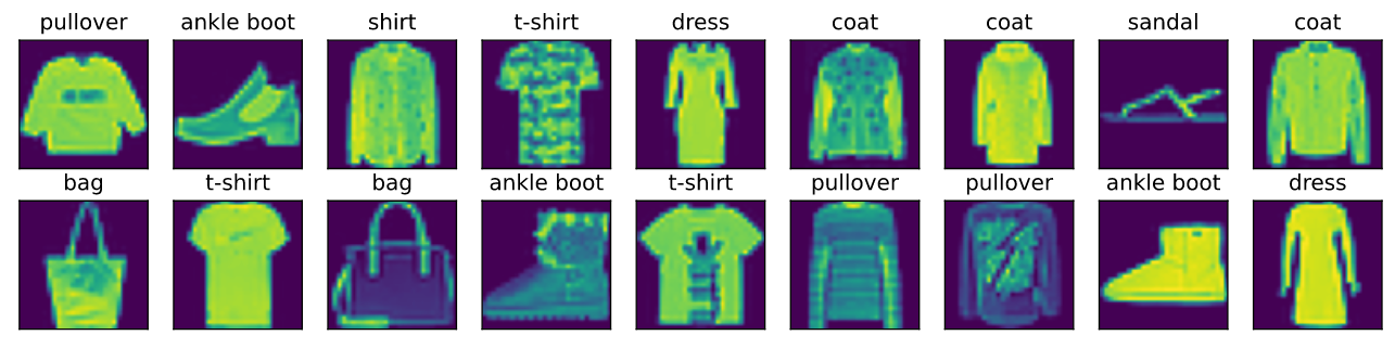
ImageNet数据集:自然物体分类(1000类)
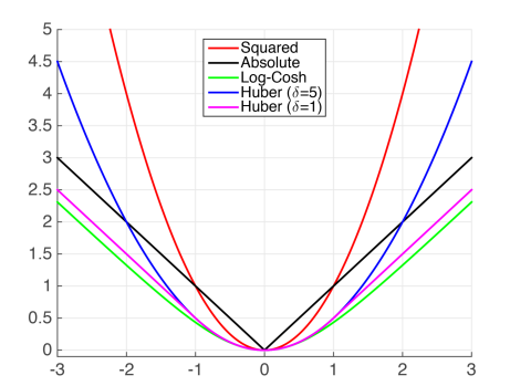
常见损失函数:
从计算角度来看,指数运算可能会造成数值稳定性问题
- softmax输入值某一类过大时,可能导致上溢(overflow),使得分子或分母变为inf(无穷大),此时解决方案是所有输入值同时减去其中最大值
- 这种幂次上的加减不会影响到最终结果,但可能导致过大的负值,从而导致下溢(underflow),容易出现反向传播中nan的情况
- 比较好的解决方案是同时计算交叉熵损失及其对数值,在反向传播中使用对数值,在计算输出概率时使用实际值
5 softmax回归实现(pytorch)
5.1 从零开始版本
import torch
from IPython import display
from d2l import torch as d2l

# 读取数据集-迭代器
batch_size = 256
train_iter, test_iter = d2l.load_data_fashion_mnist(batch_size)

num_inputs = 784 # 输入维度:28*28的图片展开长度
num_outputs = 10 # 输出维度:预测类别数
# 参数初始化
W = torch.normal(0, 0.01, size=(num_inputs, num_outputs), requires_grad=True)
b = torch.zeros(num_outputs, requires_grad=True)

def softmax(X):
    """定义softmax操作"""
    X_exp = torch.exp(X)
    partition = X_exp.sum(1, keepdim=True)
    return X_exp / partition  # 这里应用了广播机制

def net(X):
    """定义softmax回归模型"""
    # `reshape`函数将每张原始图像展平为向量
    return softmax(torch.matmul(X.reshape((-1, W.shape[0])), W) + b)

def cross_entropy(y_hat, y):
    """定义交叉熵损失函数"""
    return - torch.log(y_hat[range(len(y_hat)), y])

def accuracy(y_hat, y):  #@save
    """计算预测正确的数量"""
    if len(y_hat.shape) > 1 and y_hat.shape[1] > 1:
        y_hat = y_hat.argmax(axis=1)
    cmp = y_hat.type(y.dtype) == y
    return float(cmp.type(y.dtype).sum())

# 定义一个实用程序类,用于对多个变量进行累加
class Accumulator:  #@save
    """在n个变量上累加"""
    def __init__(self, n):
        self.data = [0.0] * n

    def add(self, *args):
        self.data = [a + float(b) for a, b in zip(self.data, args)]

    def reset(self):
        self.data = [0.0] * len(self.data)

    def __getitem__(self, idx):
        return self.data[idx]

def evaluate_accuracy(net, data_iter):
    """计算在指定数据集上模型的精度"""
    if isinstance(net, torch.nn.Module):
        net.eval()  # 将模型设置为评估模式
    metric = Accumulator(2)  # 正确预测数、预测总数
    with torch.no_grad():
        for X, y in data_iter:
            metric.add(accuracy(net(X), y), y.numel())
    return metric[0] / metric[1]

def train_epoch_ch3(net, train_iter, loss, updater):
    """训练模型一个迭代周期(定义见第3章)"""
    # 将模型设置为训练模式
    if isinstance(net, torch.nn.Module):
        net.train()
    # 训练损失总和、训练准确度总和、样本数
    metric = Accumulator(3)
    for X, y in train_iter:
        # 计算梯度并更新参数
        y_hat = net(X)
        l = loss(y_hat, y)
        if isinstance(updater, torch.optim.Optimizer):
            # 使用PyTorch内置的优化器和损失函数
            updater.zero_grad()
            l.sum().backward()
            updater.step()
        else:
            # 使用定制的优化器和损失函数
            l.sum().backward()
            updater(X.shape[0])
        metric.add(float(l.sum()), accuracy(y_hat, y), y.numel())
    # 返回训练损失和训练精度
    return metric[0] / metric[2], metric[1] / metric[2]

# 定义一个在动画中绘制数据的实用程序类-用于可视化训练进度
class Animator:
    """在动画中绘制数据"""
    def __init__(self, xlabel=None, ylabel=None, legend=None, xlim=None,
                 ylim=None, xscale='linear', yscale='linear',
                 fmts=('-', 'm--', 'g-.', 'r:'), nrows=1, ncols=1,
                 figsize=(3.5, 2.5)):
        # 增量地绘制多条线
        if legend is None:
            legend = []
        d2l.use_svg_display()
        self.fig, self.axes = d2l.plt.subplots(nrows, ncols, figsize=figsize)
        if nrows * ncols == 1:
            self.axes = [self.axes, ]
        # 使用lambda函数捕获参数
        self.config_axes = lambda: d2l.set_axes(
            self.axes[0], xlabel, ylabel, xlim, ylim, xscale, yscale, legend)
        self.X, self.Y, self.fmts = None, None, fmts

    def add(self, x, y):
        # 向图表中添加多个数据点
        if not hasattr(y, "__len__"):
            y = [y]
        n = len(y)
        if not hasattr(x, "__len__"):
            x = [x] * n
        if not self.X:
            self.X = [[] for _ in range(n)]
        if not self.Y:
            self.Y = [[] for _ in range(n)]
        for i, (a, b) in enumerate(zip(x, y)):
            if a is not None and b is not None:
                self.X[i].append(a)
                self.Y[i].append(b)
        self.axes[0].cla()
        for x, y, fmt in zip(self.X, self.Y, self.fmts):
            self.axes[0].plot(x, y, fmt)
        self.config_axes()
        display.display(self.fig)
        display.clear_output(wait=True)

def train_ch3(net, train_iter, test_iter, loss, num_epochs, updater):
    """训练模型(定义见第3章)"""
    animator = Animator(xlabel='epoch', xlim=[1, num_epochs], ylim=[0.3, 0.9],
                        legend=['train loss', 'train acc', 'test acc'])
    for epoch in range(num_epochs):
        train_metrics = train_epoch_ch3(net, train_iter, loss, updater)
        test_acc = evaluate_accuracy(net, test_iter)
        animator.add(epoch + 1, train_metrics + (test_acc,))
    train_loss, train_acc = train_metrics
    assert train_loss < 0.5, train_loss
    assert train_acc <= 1 and train_acc > 0.7, train_acc
    assert test_acc <= 1 and test_acc > 0.7, test_acc

lr = 0.1

def updater(batch_size):
    # 此处的sgd函数定义可参加第三章的2.1节的代码
    return d2l.sgd([W, b], lr, batch_size)

num_epochs = 10
train_ch3(net, train_iter, test_iter, cross_entropy, num_epochs, updater)

def predict_ch3(net, test_iter, n=6):
    """预测标签(定义见第3章)"""
    for X, y in test_iter:
        break
    trues = d2l.get_fashion_mnist_labels(y)
    preds = d2l.get_fashion_mnist_labels(net(X).argmax(axis=1))
    titles = [true +'\n' + pred for true, pred in zip(trues, preds)]
    d2l.show_images(
        X[0:n].reshape((n, 28, 28)), 1, n, titles=titles[0:n])

predict_ch3(net, test_iter)
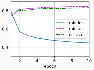
模型训练过程可视化:
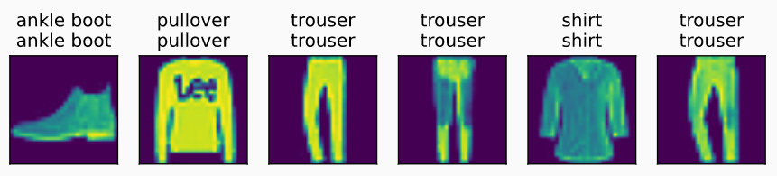
 模型最终预测结果展示:
5.2 神经网络版本
import torch
from torch import nn
from d2l import torch as d2l

# 数据读取-迭代器
batch_size = 256
train_iter, test_iter = d2l.load_data_fashion_mnist(batch_size)


# PyTorch不会隐式地调整输入的形状。因此,
# 我们在线性层前定义了展平层(flatten),来调整网络输入的形状
net = nn.Sequential(nn.Flatten(), nn.Linear(784, 10))

# 参数初始化
def init_weights(m):
    if type(m) == nn.Linear:
        nn.init.normal_(m.weight, std=0.01)
net.apply(init_weights);

loss = nn.CrossEntropyLoss() # 损失函数

trainer = torch.optim.SGD(net.parameters(), lr=0.1) # 优化算法

num_epochs = 10
# 复用从零开始版本的训练代码
d2l.train_ch3(net, train_iter, test_iter, loss, num_epochs, trainer)
6 softmax回归实现(tensorflow)
6.1 从零开始版本
import tensorflow as tf
from IPython import display
from d2l import tensorflow as d2l

# 读取数据集-迭代器
batch_size = 256
train_iter, test_iter = d2l.load_data_fashion_mnist(batch_size)

num_inputs = 784 # 输入维度:28*28的图片展开长度
num_outputs = 10 # 输出维度:预测类别数
# 参数初始化
W = tf.Variable(tf.random.normal(shape=(num_inputs, num_outputs),
                                 mean=0, stddev=0.01))
b = tf.Variable(tf.zeros(num_outputs))

def softmax(X):
    """定义softmax操作"""
    X_exp = tf.exp(X)
    partition = tf.reduce_sum(X_exp, 1, keepdims=True)
    return X_exp / partition  # 这里应用了广播机制

def net(X):
    """定义softmax回归模型"""
    # `reshape`函数将每张原始图像展平为向量
    return softmax(tf.matmul(tf.reshape(X, (-1, W.shape[0])), W) + b)

def cross_entropy(y_hat, y):
    """定义交叉熵损失函数"""
    return -tf.math.log(tf.boolean_mask(
        y_hat, tf.one_hot(y, depth=y_hat.shape[-1])))

def accuracy(y_hat, y):  #@save
    """计算预测正确的数量"""
    if len(y_hat.shape) > 1 and y_hat.shape[1] > 1:
        y_hat = tf.argmax(y_hat, axis=1)
    cmp = tf.cast(y_hat, y.dtype) == y
    return float(tf.reduce_sum(tf.cast(cmp, y.dtype)))

# 定义一个实用程序类,用于对多个变量进行累加
class Accumulator:  #@save
    """在n个变量上累加"""
    def __init__(self, n):
        self.data = [0.0] * n

    def add(self, *args):
        self.data = [a + float(b) for a, b in zip(self.data, args)]

    def reset(self):
        self.data = [0.0] * len(self.data)

    def __getitem__(self, idx):
        return self.data[idx]

def evaluate_accuracy(net, data_iter):
    """计算在指定数据集上模型的精度"""
    metric = Accumulator(2)  # 正确预测数、预测总数
    for X, y in data_iter:
        metric.add(accuracy(net(X), y), d2l.size(y))
    return metric[0] / metric[1]

def train_epoch_ch3(net, train_iter, loss, updater):
    """训练模型一个迭代周期(定义见第3章)"""
    # 训练损失总和、训练准确度总和、样本数
    metric = Accumulator(3)
    for X, y in train_iter:
        # 计算梯度并更新参数
        with tf.GradientTape() as tape:
            y_hat = net(X)
            # Keras内置的损失接受的是(标签,预测),这不同于用户在本书中的实现。
            # 本书的实现接受(预测,标签),例如我们上面实现的“交叉熵”
            if isinstance(loss, tf.keras.losses.Loss):
                l = loss(y, y_hat)
            else:
                l = loss(y_hat, y)
        if isinstance(updater, tf.keras.optimizers.Optimizer):
            params = net.trainable_variables
            grads = tape.gradient(l, params)
            updater.apply_gradients(zip(grads, params))
        else:
            updater(X.shape[0], tape.gradient(l, updater.params))
        # Keras的loss默认返回一个批量的平均损失
        l_sum = l * float(tf.size(y)) if isinstance(
            loss, tf.keras.losses.Loss) else tf.reduce_sum(l)
        metric.add(l_sum, accuracy(y_hat, y), tf.size(y))
    # 返回训练损失和训练精度
    return metric[0] / metric[2], metric[1] / metric[2]

# 定义一个在动画中绘制数据的实用程序类-用于可视化训练进度
class Animator:
    """在动画中绘制数据"""
    def __init__(self, xlabel=None, ylabel=None, legend=None, xlim=None,
                 ylim=None, xscale='linear', yscale='linear',
                 fmts=('-', 'm--', 'g-.', 'r:'), nrows=1, ncols=1,
                 figsize=(3.5, 2.5)):
        # 增量地绘制多条线
        if legend is None:
            legend = []
        d2l.use_svg_display()
        self.fig, self.axes = d2l.plt.subplots(nrows, ncols, figsize=figsize)
        if nrows * ncols == 1:
            self.axes = [self.axes, ]
        # 使用lambda函数捕获参数
        self.config_axes = lambda: d2l.set_axes(
            self.axes[0], xlabel, ylabel, xlim, ylim, xscale, yscale, legend)
        self.X, self.Y, self.fmts = None, None, fmts

    def add(self, x, y):
        # 向图表中添加多个数据点
        if not hasattr(y, "__len__"):
            y = [y]
        n = len(y)
        if not hasattr(x, "__len__"):
            x = [x] * n
        if not self.X:
            self.X = [[] for _ in range(n)]
        if not self.Y:
            self.Y = [[] for _ in range(n)]
        for i, (a, b) in enumerate(zip(x, y)):
            if a is not None and b is not None:
                self.X[i].append(a)
                self.Y[i].append(b)
        self.axes[0].cla()
        for x, y, fmt in zip(self.X, self.Y, self.fmts):
            self.axes[0].plot(x, y, fmt)
        self.config_axes()
        display.display(self.fig)
        display.clear_output(wait=True)

def train_ch3(net, train_iter, test_iter, loss, num_epochs, updater):
    """训练模型(定义见第3章)"""
    animator = Animator(xlabel='epoch', xlim=[1, num_epochs], ylim=[0.3, 0.9],
                        legend=['train loss', 'train acc', 'test acc'])
    for epoch in range(num_epochs):
        train_metrics = train_epoch_ch3(net, train_iter, loss, updater)
        test_acc = evaluate_accuracy(net, test_iter)
        animator.add(epoch + 1, train_metrics + (test_acc,))
    train_loss, train_acc = train_metrics
    assert train_loss < 0.5, train_loss
    assert train_acc <= 1 and train_acc > 0.7, train_acc
    assert test_acc <= 1 and test_acc > 0.7, test_acc

class Updater():  #@save
    """用小批量随机梯度下降法更新参数"""
    def __init__(self, params, lr):
        self.params = params
        self.lr = lr

    def __call__(self, batch_size, grads):
    	# 此处的sgd函数定义可参加第三章的3.1节的代码
        d2l.sgd(self.params, grads, self.lr, batch_size)

updater = Updater([W, b], lr=0.1)

num_epochs = 10
train_ch3(net, train_iter, test_iter, cross_entropy, num_epochs, updater)

def predict_ch3(net, test_iter, n=6):
    """预测标签(定义见第3章)"""
    for X, y in test_iter:
        break
    trues = d2l.get_fashion_mnist_labels(y)
    preds = d2l.get_fashion_mnist_labels(net(X).argmax(axis=1))
    titles = [true +'\n' + pred for true, pred in zip(trues, preds)]
    d2l.show_images(
        X[0:n].reshape((n, 28, 28)), 1, n, titles=titles[0:n])

predict_ch3(net, test_iter)
6.2 神经网络版本
import tensorflow as tf
from d2l import tensorflow as d2l

# 数据读取-迭代器
batch_size = 256
train_iter, test_iter = d2l.load_data_fashion_mnist(batch_size)

# 指定全连接层的输出维度为10并进行参数初始化
net = tf.keras.models.Sequential()
net.add(tf.keras.layers.Flatten(input_shape=(28, 28)))
weight_initializer = tf.keras.initializers.RandomNormal(mean=0.0, stddev=0.01)
net.add(tf.keras.layers.Dense(10, kernel_initializer=weight_initializer))

# 损失函数
loss = tf.keras.losses.SparseCategoricalCrossentropy(from_logits=True)

trainer = torch.optim.SGD(net.parameters(), lr=0.1) # 优化算法

num_epochs = 10
# 复用从零开始版本的训练代码
d2l.train_ch3(net, train_iter, test_iter, loss, num_epochs, trainer)