1 从全连接层到卷积层
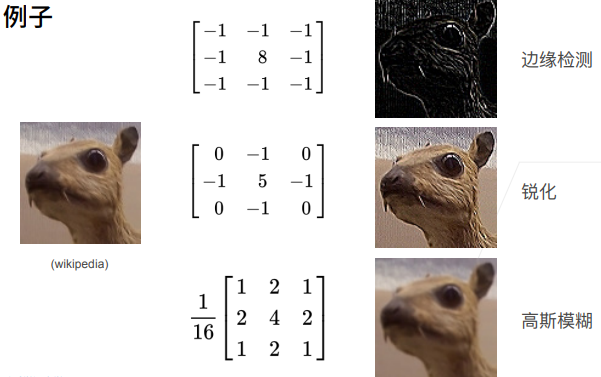
计算机视觉应具备的两个特性:
- 平移不变性(translation invariance):树上的一片叶子落到地上,它还是一片叶子
- 局部性(locality):一只眼睛和另一只眼睛在同一张脸上,才是一双眼
为了满足以上两点,神经网络引入了卷积层的概念
复习:卷积的公式定义如下:
- 连续型对象:$(f*g)(x)=\int{f(z)g(x-z)dz}$
- 离散型对象:$(f*g)(i)=\Sigma_a{f(a)g(i-a)}$
- 二维张量:$(f*g)(i,j)=\Sigma_a\Sigma_b{f(a,b)g(i-a,j-b)}$
注意区分卷积与互相关
2 图像卷积
卷积层对输入和卷积核权重进行互相关运算,并在添加标量偏置之后产生输出。
# PyTorch
import torch
from torch import nn
from d2l import torch as d2l

def corr2d(X, K):  #@save
    """计算二维互相关运算"""
    h, w = K.shape
    Y = torch.zeros((X.shape[0] - h + 1, X.shape[1] - w + 1))
    for i in range(Y.shape[0]):
        for j in range(Y.shape[1]):
            Y[i, j] = (X[i:i + h, j:j + w] * K).sum()
    return Y

# 自定义二维卷积层
class Conv2D(nn.Module):
    def __init__(self, kernel_size):
        super().__init__()
        self.weight = nn.Parameter(torch.rand(kernel_size))
        self.bias = nn.Parameter(torch.zeros(1))

    def forward(self, x):
        return corr2d(x, self.weight) + self.bias

# 卷积核`K`可以检测垂直边缘
K = torch.tensor([[1.0, -1.0]])
# Tensorflow

import tensorflow as tf
from d2l import tensorflow as d2l

def corr2d(X, K):  #@save
    """计算二维互相关运算"""
    h, w = K.shape
    Y = tf.Variable(tf.zeros((X.shape[0] - h + 1, X.shape[1] - w + 1)))
    for i in range(Y.shape[0]):
        for j in range(Y.shape[1]):
            Y[i, j].assign(tf.reduce_sum(
                X[i: i + h, j: j + w] * K))
    return Y

# 自定义二维卷积层
class Conv2D(tf.keras.layers.Layer):
    def __init__(self):
        super().__init__()

    def build(self, kernel_size):
        initializer = tf.random_normal_initializer()
        self.weight = self.add_weight(name='w', shape=kernel_size,
                                      initializer=initializer)
        self.bias = self.add_weight(name='b', shape=(1, ),
                                    initializer=initializer)

    def call(self, inputs):
        return corr2d(inputs, self.weight) + self.bias

# 卷积核`K`可以检测垂直边缘
K = tf.constant([[1.0, -1.0]])
卷积层有时被称为特征映射(feature map):一个输入映射到下一层的空间维度的转换器
感受野(receptive field):卷积神经网络每一层输出的特征图(feature map)上的像素点映射回输入图像上的区域大小。举例说明:两层$3\times3$的卷积核卷积操作之后的感受野是$5\times5$;三层$3\times3$的卷积核卷积操作之后的感受野是$7\times7$
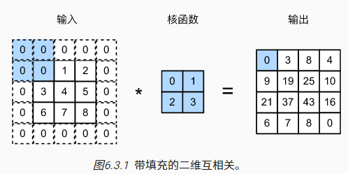
3 填充和步幅
图像边界会通过填充(padding)的方式来保证足够的空间移动卷积核
当需要保持输入输出的维度不变时,可设置填充长度=核长度-1
卷积核的高度和宽度通常为奇数,例如1、3、5或7:
- 好处1:方便左右或上下填充的对称,padding=(k-1)/2
- 好处2:奇数卷积核方便确定核中心,对边沿/线条更敏感
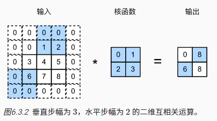
步幅(stride):卷积窗口的每次垂直/水平滑动长度(为了高效计算或缩减采样次数)
# PyTorch
import torch
from torch import nn

# 为了方便起见,我们定义了一个计算卷积层的函数。
# 此函数初始化卷积层权重,并对输入和输出提高和缩减相应的维数
def comp_conv2d(conv2d, X):
    # 这里的(1,1)表示批量大小和通道数都是1
    X = X.reshape((1, 1) + X.shape)
    Y = conv2d(X)
    # 省略前两个维度:批量大小和通道
    return Y.reshape(Y.shape[2:])

# 填充1;步幅2
conv2d = nn.Conv2d(1, 1, kernel_size=3, padding=1, stride=2)
comp_conv2d(conv2d, X).shape

# 上下不填充,左右填充1;步幅每次上下移动3,左右移动4
conv2d = nn.Conv2d(1, 1, kernel_size=(3, 5), padding=(0, 1), stride=(3, 4))
comp_conv2d(conv2d, X).shape
# Tensorflow
import tensorflow as tf

# 为了方便起见,我们定义了一个计算卷积层的函数。
# 此函数初始化卷积层权重,并对输入和输出提高和缩减相应的维数
def comp_conv2d(conv2d, X):
    # 这里的(1,1)表示批量大小和通道数都是1
    X = tf.reshape(X, (1, ) + X.shape + (1, ))
    Y = conv2d(X)
    # 省略前两个维度:批量大小和通道
    return tf.reshape(Y, Y.shape[1:3])

# filter的中心(K)与image的边角重合时开始卷积;步幅2
conv2d = tf.keras.layers.Conv2D(1, kernel_size=3, padding='same', strides=2)
comp_conv2d(conv2d, X).shape

# 当filter全部在image里面的时候,进行卷积运算;步幅每次上下移动3,左右移动4
conv2d = tf.keras.layers.Conv2D(1, kernel_size=(3,5), padding='valid',
                                strides=(3, 4))
comp_conv2d(conv2d, X).shape
4 多通道
此前分析的二维张量可看作灰度图像,彩色图像会多一个通道(channel)维度,此时卷积核也需要进行相应的维度调整:
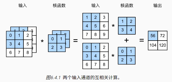
针对多输入通道的情况,每个通道都可以分别进行互相关操作,并将结果加和。
神经网络层数的加深常伴随着输出通道的维数增加,通过减少空间分辨率以获得更大的通道深度。
多输出通道情况,就是不同卷积核的叠加,每种卷积核对应着一种特征的抽取逻辑。
1 * 1卷积核
- 不再具备提取相邻像素间相关特征的能力
- 计算发生在通道间,可以看作是一个全连接层
- 常用于调整网络层的通道数量和控制模型复杂性
5 汇聚/池化层
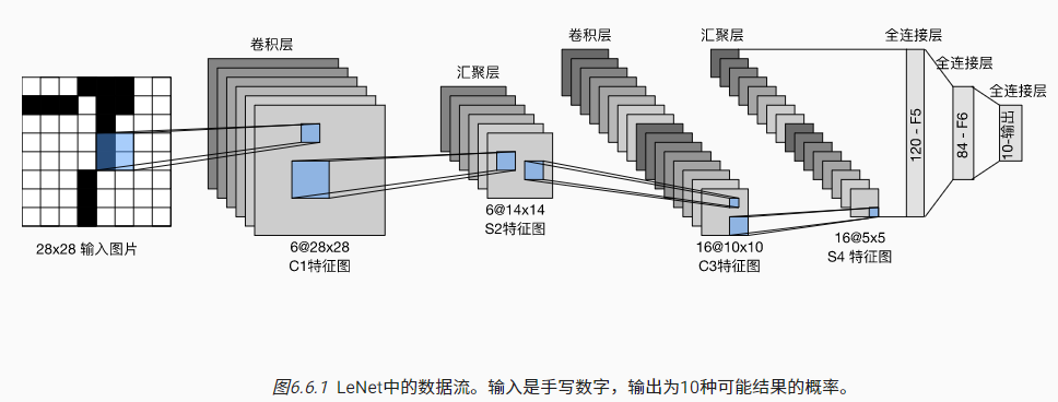
6 LeNet神经网络
LeNet,最早发布的卷积神经网络之一,由Yann LeCun在1989年提出的
主要用于手写数字识别,曾广泛用于自动取款机(ATM)机中,帮助识别处理支票的数字
代码实现(PyTorch):
# PyTorch 实现LeNet并应用于Fashion-MNIST
import torch
from torch import nn
from d2l import torch as d2l
# 相比于原版,去掉了最后一层的高斯激活
net = nn.Sequential(
nn.Conv2d(1, 6, kernel_size=5, padding=2), nn.Sigmoid(),
nn.AvgPool2d(kernel_size=2, stride=2),
nn.Conv2d(6, 16, kernel_size=5), nn.Sigmoid(),
nn.AvgPool2d(kernel_size=2, stride=2),
nn.Flatten(),
nn.Linear(16 * 5 * 5, 120), nn.Sigmoid(),
nn.Linear(120, 84), nn.Sigmoid(),
nn.Linear(84, 10))
X = torch.rand(size=(1, 1, 28, 28), dtype=torch.float32)
for layer in net: # 打印输出每一层的维度
X = layer(X)
print(layer.__class__.__name__,'output shape: \t',X.shape)
def evaluate_accuracy_gpu(net, data_iter, device=None): #@save
"""使用GPU计算模型在数据集上的精度"""
if isinstance(net, nn.Module):
net.eval() # 设置为评估模式
if not device:
device = next(iter(net.parameters())).device
# 正确预测的数量,总预测的数量
metric = d2l.Accumulator(2)
with torch.no_grad():
for X, y in data_iter:
if isinstance(X, list):
# BERT微调所需的(之后将介绍)
X = [x.to(device) for x in X]
else:
X = X.to(device)
y = y.to(device)
metric.add(d2l.accuracy(net(X), y), y.numel())
return metric[0] / metric[1]
#@save
def train_ch6(net, train_iter, test_iter, num_epochs, lr, device):
"""用GPU训练模型(在第六章定义)"""
def init_weights(m):
if type(m) == nn.Linear or type(m) == nn.Conv2d:
nn.init.xavier_uniform_(m.weight)
net.apply(init_weights)
print('training on', device)
net.to(device)
optimizer = torch.optim.SGD(net.parameters(), lr=lr)
loss = nn.CrossEntropyLoss()
animator = d2l.Animator(xlabel='epoch', xlim=[1, num_epochs],
legend=['train loss', 'train acc', 'test acc'])
timer, num_batches = d2l.Timer(), len(train_iter)
for epoch in range(num_epochs):
# 训练损失之和,训练准确率之和,样本数
metric = d2l.Accumulator(3)
net.train()
for i, (X, y) in enumerate(train_iter):
timer.start()
optimizer.zero_grad()
X, y = X.to(device), y.to(device)
y_hat = net(X)
l = loss(y_hat, y)
l.backward()
optimizer.step()
with torch.no_grad():
metric.add(l * X.shape[0], d2l.accuracy(y_hat, y), X.shape[0])
timer.stop()
train_l = metric[0] / metric[2]
train_acc = metric[1] / metric[2]
if (i + 1) % (num_batches // 5) == 0 or i == num_batches - 1:
animator.add(epoch + (i + 1) / num_batches,
(train_l, train_acc, None))
test_acc = evaluate_accuracy_gpu(net, test_iter)
animator.add(epoch + 1, (None, None, test_acc))
print(f'loss {train_l:.3f}, train acc {train_acc:.3f}, '
f'test acc {test_acc:.3f}')
print(f'{metric[2] * num_epochs / timer.sum():.1f} examples/sec '
f'on {str(device)}')
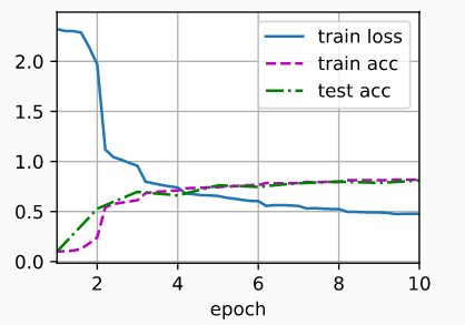
lr, num_epochs = 0.9, 10
train_ch6(net, train_iter, test_iter, num_epochs, lr, d2l.try_gpu())D
# loss 0.476, train acc 0.820, test acc 0.812
# 103100.0 examples/sec on cuda:0
代码实现(Tensorflow):
# Tensorflow 实现LeNet并应用于Fashion-MNIST
import tensorflow as tf
from d2l import tensorflow as d2l

# 相比于原版,去掉了最后一层的高斯激活
def net():
    return tf.keras.models.Sequential([
        tf.keras.layers.Conv2D(filters=6, kernel_size=5, activation='sigmoid',
                               padding='same'),
        tf.keras.layers.AvgPool2D(pool_size=2, strides=2),
        tf.keras.layers.Conv2D(filters=16, kernel_size=5,
                               activation='sigmoid'),
        tf.keras.layers.AvgPool2D(pool_size=2, strides=2),
        tf.keras.layers.Flatten(),
        tf.keras.layers.Dense(120, activation='sigmoid'),
        tf.keras.layers.Dense(84, activation='sigmoid'),
        tf.keras.layers.Dense(10)])

X = tf.random.uniform((1, 28, 28, 1))
for layer in net().layers:
    X = layer(X) # 打印输出每一层的维度
    print(layer.__class__.__name__, 'output shape: \t', X.shape)

batch_size = 256
train_iter, test_iter = d2l.load_data_fashion_mnist(batch_size=batch_size)

class TrainCallback(tf.keras.callbacks.Callback):  #@save
    """一个以可视化的训练进展的回调"""
    def __init__(self, net, train_iter, test_iter, num_epochs, device_name):
        self.timer = d2l.Timer()
        self.animator = d2l.Animator(
            xlabel='epoch', xlim=[1, num_epochs], legend=[
                'train loss', 'train acc', 'test acc'])
        self.net = net
        self.train_iter = train_iter
        self.test_iter = test_iter
        self.num_epochs = num_epochs
        self.device_name = device_name

    def on_epoch_begin(self, epoch, logs=None):
        self.timer.start()

    def on_epoch_end(self, epoch, logs):
        self.timer.stop()
        test_acc = self.net.evaluate(
            self.test_iter, verbose=0, return_dict=True)['accuracy']
        metrics = (logs['loss'], logs['accuracy'], test_acc)
        self.animator.add(epoch + 1, metrics)
        if epoch == self.num_epochs - 1:
            batch_size = next(iter(self.train_iter))[0].shape[0]
            num_examples = batch_size * tf.data.experimental.cardinality(
                self.train_iter).numpy()
            print(f'loss {metrics[0]:.3f}, train acc {metrics[1]:.3f}, '
                  f'test acc {metrics[2]:.3f}')
            print(f'{num_examples / self.timer.avg():.1f} examples/sec on '
                  f'{str(self.device_name)}')

#@save
def train_ch6(net_fn, train_iter, test_iter, num_epochs, lr, device):
    """用GPU训练模型(在第六章定义)"""
    device_name = device._device_name
    strategy = tf.distribute.OneDeviceStrategy(device_name)
    with strategy.scope():
        optimizer = tf.keras.optimizers.SGD(learning_rate=lr)
        loss = tf.keras.losses.SparseCategoricalCrossentropy(from_logits=True)
        net = net_fn()
        net.compile(optimizer=optimizer, loss=loss, metrics=['accuracy'])
    callback = TrainCallback(net, train_iter, test_iter, num_epochs,
                             device_name)
    net.fit(train_iter, epochs=num_epochs, verbose=0, callbacks=[callback])
    return net

lr, num_epochs = 0.9, 10
train_ch6(net, train_iter, test_iter, num_epochs, lr, d2l.try_gpu())
#loss 0.467, train acc 0.824, test acc 0.812
#53671.6 examples/sec on /GPU:0
结果表现: